The Influencer selection problem
Advertisers using influencer posts to promote products and services have a big problem called targeting. If an advertiser advertises, for example, through Google Ads, he can focus on an arbitrarily narrow thematic audience segment that exactly matches the goods and services that he is promoting to the market.
There is no such possibility on social networks: there are millions of potential influencers on Instagram where you can advertise. How to choose from them those whose thematics suit the advertiser? Either the advertiser must actively use Instagram himself and a priori know those bloggers who are suitable for him (i.e. only large ones and only those to whom he himself is subscribed), or just give ads at random, hoping that they will reach at least a small percentage of the target audience.
It is clear that both options are not very good, so Instagram is not very effective for “niche” medium and small advertisers.
If this problem is solved, advertising on Instagram will become accessible and convenient for everyone, not just for big brands.
Tree-like hierarchy of topics? No, thanks.
The most obvious way to associate influencers with topics is through a tree-like hierarchy of topics. To do this, a topic hierarchy should be carefully thought out at first. Each influencer is then manually (or with help of some ML model) assigned to the nodes of this hierarchy.
Most advertising systems go this way, including such large ones as Facebook Ads. But in fact, this is an inefficient solution. The number of topics potentially interesting to advertisers is very large. It would not be a mistake to say that it is potentially infinite: the more narrow the advertising niche, the finer division into topics is required.
- For example, there is a topic Food.
- It is obvious that the restaurant needs not only Food, but Food : Restaurants.
- If this is a Thai restaurant, then an even narrower topic is needed: Food : Restaurants : Thai cuisine.
- If this restaurant is located in London, it would be nice to add the topic Food : Restaurants : London, etc.
But the topic hierarchy cannot grow indefinitely:
- It will become trivially inconvenient for the advertiser to work with such a large hierarchy. The size of a hierarchy that an ordinary person can effortlessly perceive and keep in his head is no more than 100 nodes.
- The more topics, the more difficult it is to attribute a blogger to specific topics and the more work is needed for this. It is generally impossible to do this work manually (there are several million bloggers). Of course, it’s possible to use machine learning, but you still need to make a training dataset first, i.e. examples of the correct matches between topics and bloggers. Dataset is made up of people, people make mistakes, people are subjective in their views and assessments (different assessors will attribute the same blogger to different topics).
- You will have to spend a lot of effort on keeping the topics hierarchy up to date (new trends are constantly appearing, new topics are being opened and old ones are dying off), and on updating the training dataset.
It turns out that a small hierarchy of topics will be too inflexible and give too coarse segments, while at the same time a large hierarchy will be inconvenient to work with. Another solution is needed.
The thematics is set by the advertiser
What if the thematics could be defined with a set of keywords, like in Google Ads? Then the advertiser will be able to set up for himself any arbitrarily narrow thematics, and at the same time he will not have to crawl through a huge topic hierarchy. But in Google Ads, the keywords correspond to what potential customers are explicitly looking for, and what should the keywords in Instagram correspond to? Hashtags? But it’s not that simple.
- A blogger writing about cars will not necessarily use the hashtag
#car, he can use#auto,#fastcars,#wheels,#driveor brand names#bmw,#audi, etc. How is an advertiser supposed to guess what specific tags bloggers are using? In principle, the same problem exists in Google Ads: the advertiser must make considerable efforts to cover all possible keywords in his subject. - A blogger might accidentally use a hashtag like
#carif he bought a new car, or just saw and photographed an interesting car on the street. This does not mean at all that he writes on automotive topics. - Bloggers often use popular tags that have nothing to do with the topic of the post, just to get into the search results for the tag (hashtag spam).
For example, the tag
#catcan be marked with a photo of a bearded hipster, a landscape with a sunset, or a selfie of yourself in a new outfit and surrounded by friends.
Therefore, the selection of bloggers simply by the presence of tags set by the advertiser will not work well. We need more intelligent ways to solve this problem.
Topic modeling, theory
In modern natural language processing techniques, there is an approach called topic modeling. It is easiest to explain the application of topic modeling to our problem with a simple example.
Let’s imagine a very primitive social network in which people have only two main interests - interest in Food, and interest in Japan. If interest strength is given by a number from 0 to 1, then any hashtags used by bloggers can be placed on a 2D chart.
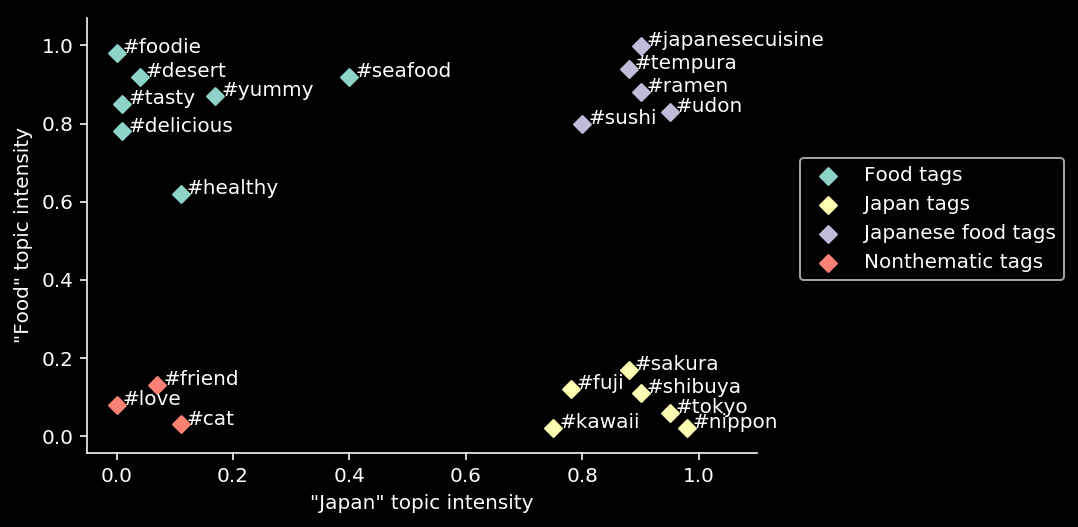
Example of 2D topic space
It can be seen that any hashtag can be described by a pair of numbers corresponding to the X and Y coordinates in the thematic space. Tags related to the same topic are grouped into clusters, i.e. they have close coordinates. Using this chart, it’s possible to calculate the relevance of a post to topics. We have to calculate, by all tags in the post, its “averaged” coordinates in the topic space (i.e., calculate centroid). The centroid coordinates along the X and Y axes will correspond to the relevance of the post to Food and Japan topics. The closer the coordinate is to 1, the higher the relevance. In the same way, by calculating the centroid of all blogger posts, it is possible to understand which topics the blogger’s content is generally relevant to.
In real topic modeling, of course, tens and hundreds of topics are used, not two. Accordingly, tags have to be defined in high-dimensional space instead of 2D. More precise definition:
- There is a set of documents $D$ (in our case these are posts), a set of words $W$ (in our case tags) and a set of topics $T$, the size of which is predetermined.
- The content of documents can be represented as a set of document-word pairs: $(d, w), d \in D, w \in W_d$
- Each topic $t \in T$ is described by an unknown distribution $p(w|t)$ over set of words $w \in W$
- Each document $d\in D$ is described by an unknown distribution $p(t|d)$ over set of topics $t\in T$
- It is assumed that the distribution of words in documents depends only on the subject: $p(w|t,d)=p(w|t)$
- In the process of building a topic model, the algorithm finds the “word–topic” matrix $\mathbf{\Phi} =||p(w|t)||$ and the “topic–document” matrix $\mathbf{\Theta} =| |p(t|d)||$ by the contents of the collection $D$. We are interested in the first matrix.
Topic modeling is equivalent to Non-negative matrix factorization The input contains a sparse “word-document” matrix $\mathbf{S} \in \mathbb{R}^{W \times D}$, which describes the probability of encountering the word $w$ in document $d$. Its approximation is calculated as a product of low-rank matrices $\mathbf{\Phi} \in \mathbb{R}^{W \times T}$ and $\mathbf{\Theta} \in \mathbb{R}^{T \times D}$. $$\mathbf{S} \approx \mathbf{\Phi}\mathbf{\Theta}$$ For more information on topic modeling, see Wikipedia.
Topic modeling, practice
In practice, thematic modeling produced mediocre results. The table below shows the results of modeling on 15 topics using the BigARTM library:
| Topic | Top tags |
|---|---|
| 0 | sky, clouds, sea, spring, baby, ocean, nyc, flower, landscape, drinks |
| 1 | beer, vintage, chill, school, rainbow, yoga, rock, evening, chicago, relaxing |
| 2 | sweet, chocolate, dance, rain, nike, natural, anime, old, wcw, reflection |
| 3 | foodporn, breakfast, delicious, foodie, handmade, gold, instafood, garden, healthy, vegan |
| 4 | architecture, california, lights, portrait, newyork, wine, blonde, familytime, losangeles, thanksgiving |
| 5 | nature, travel, autumn, london, fall, trees, tree, photoshoot, city, cake |
| 6 | flowers, design, inspiration, artist, goals, illustration, pizza, ink, glasses, money |
| 7 | winter, snow, catsofinstagram, sexy, cats, cold, quote, fire, disney, festival |
| 8 | work, mountains, paris, football, nails, video, florida, diy, free, japan |
| 9 | dog, puppy, wedding, dogsofinstagram, dogs, roadtrip, painting, trip, thankful, pet |
| 10 | coffee, quotes, river, yum, moon, streetart, sleepy, music, adidas, positivevibes |
| 11 | style, fashion, party, home, model, music, dress, goodvibes, couple, tired |
| 12 | fitness, motivation, gym, workout, drawing, dinner, fit, sketch, health, fresh |
| 13 | beach, lake, usa, shopping, hiking, fashion, kids, park, freedom, sand |
| 14 | makeup, cat, yummy, eyes, snapchat, homemade, tattoo, kitty, lips, mom |
It can be seen that some kind of reasonable structure can be traced, but the topics are far from perfect. Increasing the number of topics to 150 gives a relatively small improvement.
Perhaps the reason is that topic modeling is designed to work with documents containing hundreds or thousands of words. In our case, most posts have only 2-3 tags. Other libraries ( Gensim, Mallet) also showed very modest results.
Therefore, a different, simpler and at the same time more powerful modeling method was chosen. $ \newcommand{\sim}[2]{\operatorname{sim}(#1,#2)} $
TopicTensor model
The main advantage of thematic modeling is the interpretability of the results obtained. For any word/tag, the output is a set of weights showing how close this word is to each topic from the entire set.
But this plus imposes serious restrictions on the model, forcing it to fit strictly into a fixed number of topics, no more and no less. In real life, the number of topics of a large social network is almost infinite. Therefore, if we remove the requirement for the interpretability of topics (and their fixed number), model will become more effective.
The result is a model close to the well-known Word2Vec model. Each tag is represented as a vector in $N$-dimensional space: $w \in \mathbb{R}^N$. The degree of similarity (i.e. how close the topics are) between $w$ and $w’$ tags can be calculated as a dot product: $$\sim{w}{w’}=w \cdot w’$$ as Euclidean distance: $$\sim{w}{w’}=\|w-w’\|$$ as cosine similarity: $$\sim{w}{w’}=\cos(\theta )=\frac{w \cdot w’}{\|w \|\|w’ \|}$$
The task of the model during training is to find such representations of tags that will be useful for one of the predictions:
- Based on a single tag, predict what other tags will be included in a post (Skip-gram architecture)(Edited)Restore original
- Based on all post tags except one, predict the missing tag (CBOW architecture, “bag of words”)
- Take two random tags from a post and predict the second based on the first one
All these predictions come down to the fact that there is a target tag $w_t$ to be predicted, and a context $c$ represented by one or more tags included in the post. The model should maximize the probability of a tag depending on the context, this can be represented as a softmax criterion:
$$P(w_t|c) = \operatorname{softmax}(\sim{w_t}{c})$$ $$P(w_t|c) = \frac{\exp(\sim{w_t}{c})}{\sum_{w’ \in W}\exp(\sim{w’}{c})}$$
But calculating softmax over the entire set of $W$ tags is expensive (millions of tags may be involved in training), so alternative methods are used instead. They boil down to the fact that there is a positive example $(w_t,c)$ to be predicted, and randomly chosen negative examples $(w_1^{-}, c), (w_2^{-}, c),\dots,(w_n^{-}, c)$ being an example of how not to predict. Negative examples should be sampled from the same tag frequency distribution as in the training data.
Loss function for a set of examples can be in the form of a binary classification (Negative sampling in the classic Word2Vec) $$L = \log(\sigma(\sim{w_t}{c})) + \sum_i\log(\sigma(-\sim{w_i^-}{c}))$$ $$\sigma(x) = \frac{1}{1+e^{-x}}$$ or work like a ranking loss, pairwise comparing “compatibility” with the context of positive and negative examples: $$L = \sum_{i} l(\sim{w_t}{c}, \sim{w_i^-}{c})$$ where $l(\cdot, \cdot)$ is a ranking function, for example max margin loss: $$l=\max(0,\mu+\sim{w_i^-}{c}−\sim{w_t}{c})$$
The TopicTensor model is also equivalent to the matrix factorization, but instead of the “document-word” matrix (as in topic modeling), the “context-tag” matrix is ised. For some types of predictions, it turns into a matrix of mutual occurrence of tags “tag-tag”.
Implementation of TopicTensor
Several possible ways to implement the model have been considered: Custom code using Tensorflow, custom code using PyTorch, Gensim library, [StarSpace] https://github.com/facebookresearch/StarSpace) library. The last option was chosen as requiring minimal effort (all the necessary functionality is already there), producing high quality topics, and almost linearly parallelized on any number of cores (32 and 64-core machines were used to speed up learning).
StarSpace by default uses max margin ranking loss as loss function and cosine distance as the proximity metric for vectors. Subsequent experiments with hyperparameters have shown that these default settings are optimal.
Hyperparameter tuning
Before the final training, hyperparameters were tuned in order to find a balance between quality and acceptable training time.
The quality was measured as follows: a set of posts was taken that the model did not see during the training. For each tag from the post (a total of $n$ tags in the post), the candidate tags closest to it were selected according to the cosine similarity criterion from the set of all $W$ tags: $$candidates_i=\operatorname{top_n}(\sim{w_t}{w’}, \forall w’ \in W)$$ $$i \in 1 \dots n$$ It was calculated how many of these candidates matched the real tags in the post (number of matches $n^{+}$). $$quality=\frac{\sum n^+}{\sum n}$$ Quality is the percentage of correctly matched tags for all posts from the sample.
This method of quality assessment also implies that it is most optimal to train the model according to the skip-gram criterion (predict the rest of the tags by one tag). This was confirmed in practice: skip-gram training showed the best quality, although it turned out to be the slowest.
The following hyperparameters were tuned:
- Dimension of topic vectors
- Number of training epochs
- Number of negative examples
- Learning rate
Подготовка данных
Tags have been normalized: reduced to lowercase, diacritics removed.
The tags that were used by at least N different bloggers were selected to provide a diversity of usage contexts (depending on the language, N varied from 20 to 500).
For each language, a list of top 1000 most frequent tags was made. From this list, commonly used words that do not carry a thematic meaning (me, you, together, etc), numerals, color names (red, yellow, etc.), and some tags especially loved by spammers were blacklisted.
Each blogger’s tags are reweighted according to how often they are used by that blogger. Most bloggers have “favorite” tags that are used in almost every post, and if such tags are not weighted down, an active blogger can skew the global statistics of tag co-occurency and the model will be biased.
The final traininbg dataset consisted of about 8 billion tags out of 1 billion posts. Training took over three weeks on a 32-core server.
Results
The obtained embeddings had excellent topic separation, good generalization ability, and resistance to spam tags.
Demo sample of top 10K tags is available for viewing
in Embedding Projector. After clicking on the link, you need to switch to the UMAP ot T-SNE mode
(tab in the lower left part) and wait until the 3D projection is built. It’s better to view projection in Color By = logcnt mode.
Examples of topic formation
Let’s start with the simplest. Let’s set the topic with one tag and find the top 50 relevant tags.
Topic set by tag 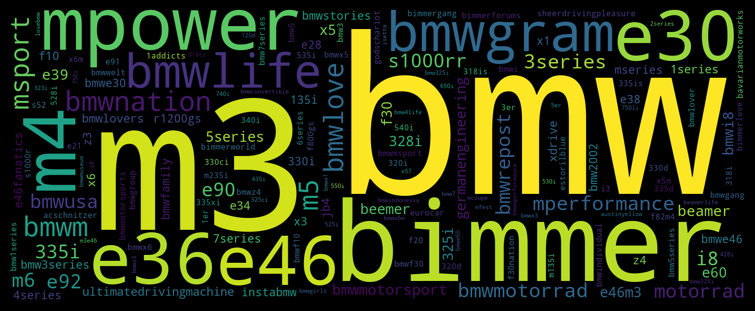
#bmw
 Tags are colored according to relevance. The size of a tag is proportional to its popularity.
As you can see, TopicTensor has done a great job building the ‘BMW’ thematics and found a lot of relevant tags that most people don’t even know exist.
Let’s complicate the task and buuld the topic of several German auto brands:
Topic set by tags 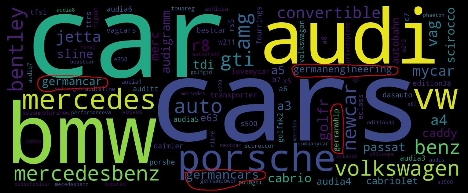
#bmw, #audi, #mercedes, #vw
This example shows TopicTesnor’s ability to generalize:
TopicTensor understood that we mean cars in general (tags #car, #cars).
The model also realized that it was necessary to give preference to German cars (tags circled in red),
and added “missing” tags: #porsche (also a German car brand),
as well as spellings of tags that were not in the input: #mercedesbenz , #benz and #volkswagen
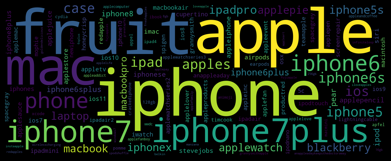
Topic set by tag #apple
Let’s complicate the task even more and create a theme based on the ambiguous #apple tag, which can mean both a brand
and just a fruit. It can be seen that the brand theme dominates, however, the fruit theme is also present in the form
of #fruit, #apples and #pear tags.
Let’s try to highlight a pure “fruit” theme, for this we will add several tags related to the apple brand, with a negative weight. Accordingly, we will try to find tags that are closest (in embedding space) to the weighted sum of input tag embeddings (by default, the weight is equal to one): $$target = \sum_i w_i \cdot tag_i $$
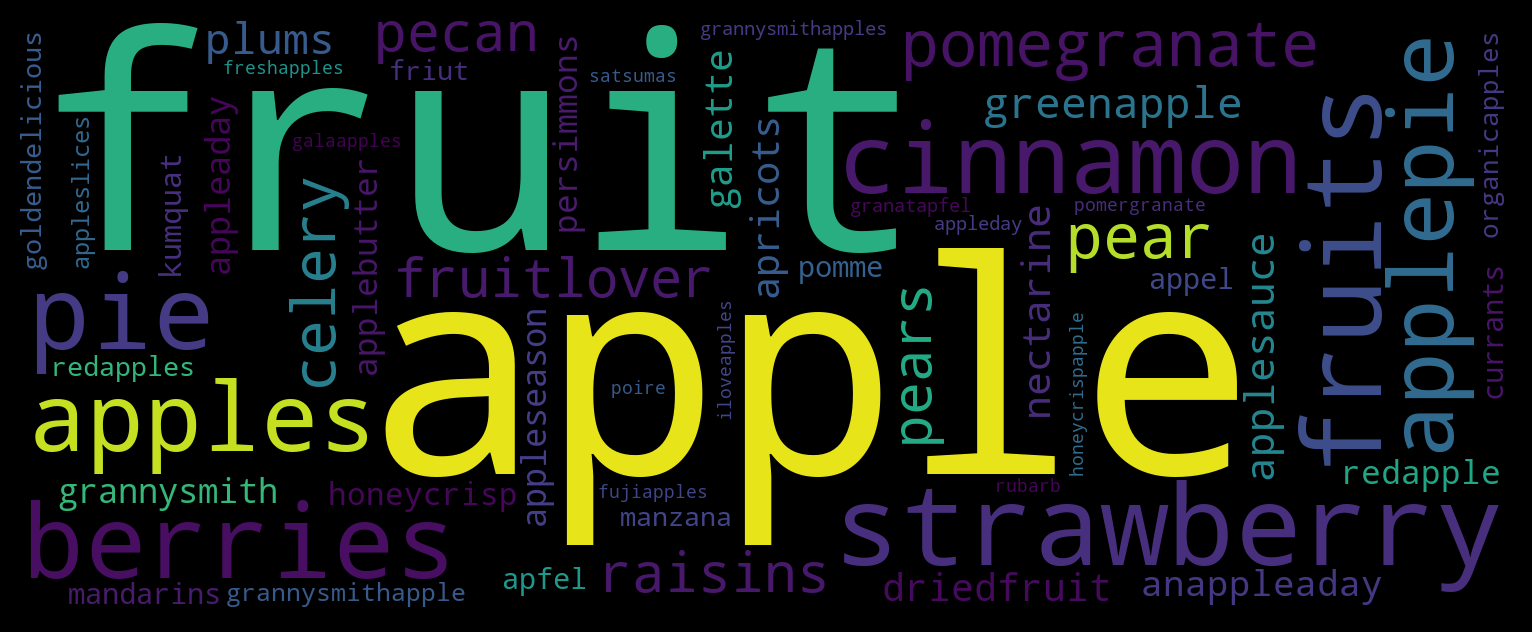
Topic set by tags #apple, #iphone:-1, #macbook:-0.05 #macintosh:-0.005
It can be seen that the negative weights removed the brand theme, and only the fruit theme remained.
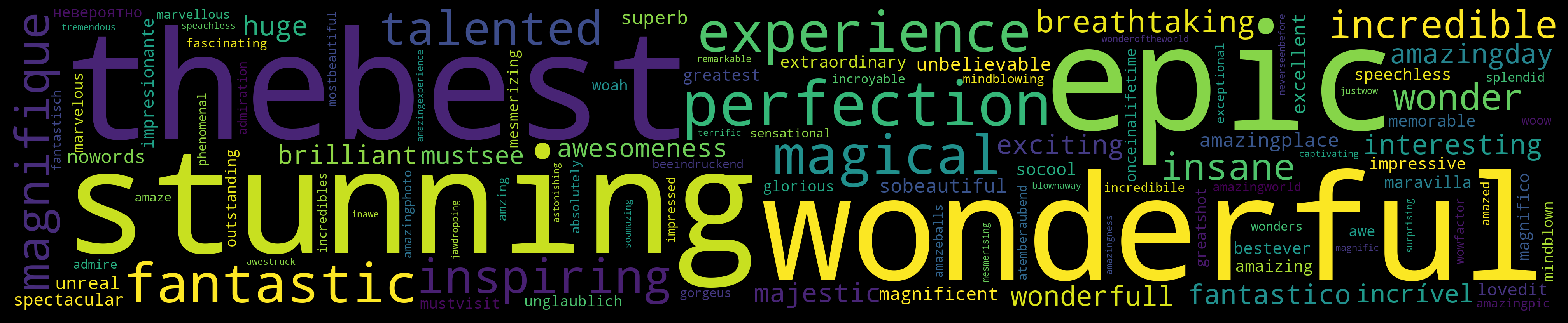
Тopic set by tag 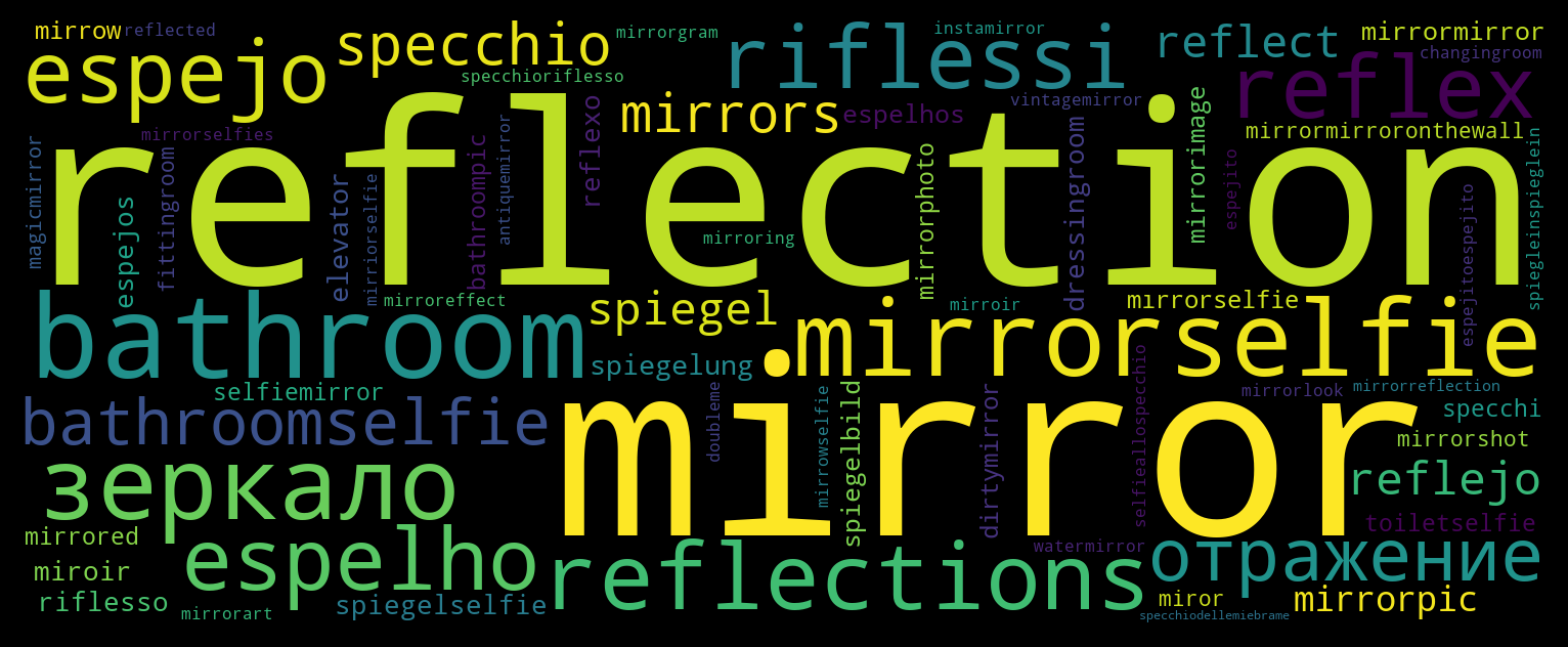
#mirror
#mirror example.
Found tags that express the same concept:
mirror and reflection in English, зеркало and отражение in Russian,
espejo and reflejo in Spanish, espelho and reflexo in Portuguese,
specchio and riflesso in Italian, spiegel and spiegelung in German.
Тopic set by tag 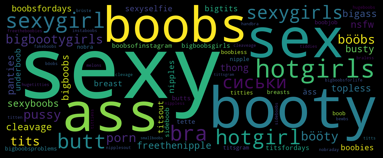
#boobs
Blogger selection
For each blogger, all his posts are analyzed and the embeddings of all used tags are summarized. $$\beta=\sum_i^{|posts|}\sum_j^{|tags_i|} w_{ij}$$ where $|posts|$ is the number of posts, $|tags_i|$ is the number of tags in the $i$th post. The resulting vector $\beta$ is the topic of the blogger. Then the system selects bloggers whose topic vector is closest to the topic vector specified by the user via tags. The bloger list is sorted by relevance and issued to the user.
Additionally, the popularity of the blogger and the number of tags in his posts are taken into account. The final score, by which bloggers are sorted, is calculated as follows: $$score_i = {\sim{input}{\beta_i} \over \log(likes)^\lambda \cdot \log(followers)^\phi \cdot \log(tags)^\tau}$$ where $\lambda, \phi, \tau$ are empirically chosen coefficients lying in the interval $0\dots1$
Calculatiion of cosine distance across the entire array of bloggers (several million accounts) takes a significant amount of time. To speed up the blogger selection, the library [NMSLIB (https://github.com/nmslib/nmslib) (Non-Metric Space Library) was used. It reduces the selection time by an order of magnitude due to usage of multidimensional indexes.
Demo site
A demo site with a limited number of tags and bloggers is available at http://tt-demo.suilin.ru/. On this site, you can experiment on your own with the formation of topics and blogger selection.
Thematic lookalikes
The $\beta$ vectors calculated for blogger selection can also be used to match similair bloggers with each other. In fact, lookalike matching is not much different from blogger selection. The only difference is the input: instead of a topic vector calculated as sum of tag embeddings, the topic vector $\beta$ of a specified blogger is given as input. The output is a list of bloggers whose thematics are close to those of a given blogger, in order of relevance.
Фиксированные тематики
As already mentioned, there are no explicitly defined topics in TopicTensor. However, for some tasks we do need to have an explicit set/hierarchy of most prominent topics across all posts/bloggers. In other words, we need to extract most important topics from a vector space of tag embeddings.
Самый очевидный способ экстракции тематик это кластеризация векторного представления тэгов, один кластер = одна тематика. Кластеризация проводилась в два этапа, т.к. алгоритмов, способных эффективно искать кластера в 200D пространстве, пока не существует.
The most obvious way to extract topics is to cluster the tag embeddings, one cluster = one topic. Clustering was carried out in two stages, because algorithms that can efficiently search for a cluster in 200D space do not yet exist.
At the first stage, dimensionality reduction was carried out using the [UMAP] library (https://github.com/lmcinnes/umap). The dimension was reduced to 5D, cosine distance was used as a distance metric, the values of remaining hyperparameters were selected based on the results of clustering (second stage).
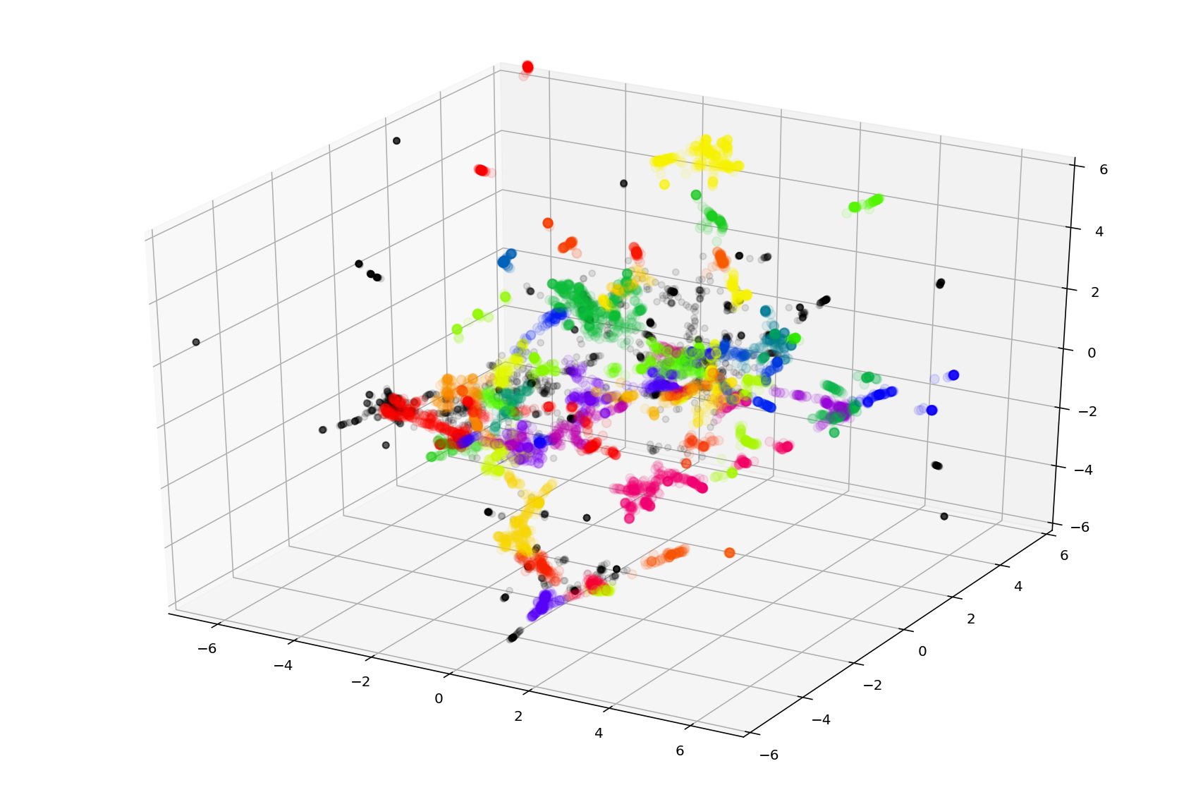
An example of tag clustering in 3D space. Different clusters are marked with different colors (colors are not unique and may be repeated for different clusters).
At the second stage, clustering was carried out using the HDBSCAN algorithm. Clustering results (English only) can be seen on GitHub. Clustering identified about 500 topics (it’s possible to adjust the number of topics within a wide range using UMAP and HDBSCAN hyperparameters).
Inspection showed good topic coherence and no noticeable correlation between clusters. However, for the practical application, clusters need to be improved: remove useless ones (e.g. private name cluster, negative emotion cluster, common words cluster), merge some close clusters.